Access and Plot measurements

The following code shows how to load and plot measurements of a LinearAccelerationSeries and a GPSSeries.

import logging
import numpy as np
import matplotlib.pyplot as plt
import matplotlib.dates as mdates

from scipy import signal

import pyridy

from pyridy.utils import AccelerationSeries, LinearAccelerationSeries, NTPDatetimeSeries, GyroSeries, GPSSeries, MagnetometerSeries # Every data series that should be used should be imported here

The argument download_osm_data tries to download additional OSM which includes: railway track data, railway lines, position of level crossings and switches. Sometimes the Overpass API which is used to access the data can be overloaded leading to an error.

path = "../ridy_data"
# Load only some timeseries
campaign = pyridy.Campaign(folder=path,sync_method="ntp_time", download_osm_data=True, railway_types=["rail"], osm_recurse_type=">")

WARNING:pyridy.file:(2021-10-23T183518.175+0200d.sqlite) No NTP timestamp and datetime, falling back to device_time synchronization

[WinError 10061] No connection could be made because the target machine actively refused it
[WinError 10061] No connection could be made because the target machine actively refused it

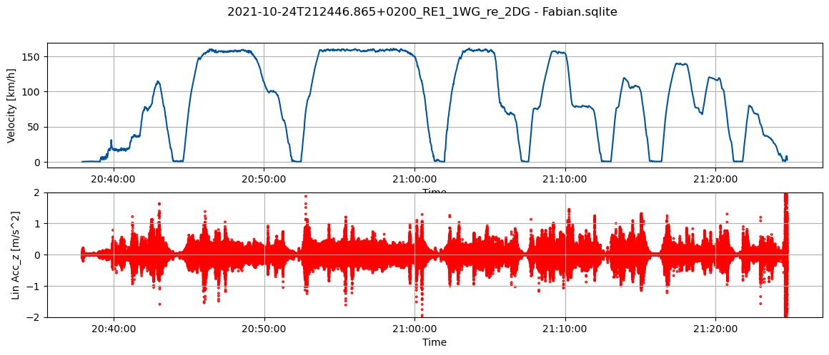
The following code plots the velocity and linear acceleration of one vehicle over time. Due to the long measurement duration, it can take a few seconds until the plot appears.

f = campaign[1] # Individual files can either be accessed over indices or by calling the campaign with the file name campaign("NAME_OF_THE_FILE")

fig, ax = plt.subplots(2, 1, sharex="row", figsize=(14, 5))

# Upper plot showing vehicle speed
ax[0].plot(f.measurements[GPSSeries].time, f.measurements[GPSSeries].speed*3.6)  # Note that individual data series can be accessed using their classes which have to be imported before
ax[0].grid()
ax[0].set_ylabel("Velocity [km/h]")
ax[0].set_xlabel("Time")
ax[0].xaxis.set_major_formatter(mdates.DateFormatter('%H:%M:%S'))

# Lower plot showing vehicle vertical acceleration
ax[1].scatter(f.measurements[LinearAccelerationSeries].time, f.measurements[LinearAccelerationSeries].lin_acc_z, facecolors='none', edgecolors='r',s=3)
ax[1].grid()
ax[1].set_ylabel("Lin Acc_z [m/s^2]")
ax[1].set_xlabel("Time")
ax[1].set_ylim(-2, 2)
ax[1].xaxis.set_major_formatter(mdates.DateFormatter('%H:%M:%S'))


plt.suptitle(f.filename)
plt.show()